

TOPCAT is a GUI desktop table manipulation application for working with tabular data, and STILTS is its command-line counterpart. These applications can work with the output from GaiaXPy, including plotting spectra.
TOPCAT can plot columns containing arrays such as spectra using the XYArray layer control from its Plane Plot window. This requires you to supply expressions that give, for each row in the table, matching arrays of X and Y values, so that one spectrum is plotted for each table row. For GaiaXPy output, the Y values are usually given by one of the array-valued columns such as flux, while the X (wavelength-like) values are supplied as an array-valued table parameter - an item of per-table metadata that can be seen in the Parameters Window - with the name "sampling". This can be referenced in TOPCAT's expression language, and hence specified for plotting, by writing "param$sampling".
If you select a GaiaXPy output file for plotting in the XYArray layer control, TOPCAT will usually fill in these values for you, but you can adjust the default settings, for instance to plot a different array-valued column from the table, include error bars, add mean/median/quantile spectra summarising all plotted rows, or perform algebraic manipulation on the input spectrum or sampling arrays.
Its underlying table processing facilities are provided by the related packages STIL and STILTS.
More information about TOPCAT (including downloads) can be found here. Note that some of the functionality described on this page requires a recent version of the software; TOPCAT v4.8-5/STILTS v3.4-5 (10 June 2022) or later are recommended.
TOPCAT can read any file produced by GaiaXPy. Although, only the output of any GaiaXPy tool that requires/produces a sampling can be plotted as spectra.
To plot GaiaXPy data, the sampling needs to be included in the file, which is the case with FITS and VOTable (XML) files. CSV and ECSV files cannot be used for plotting as the sampling comes as a separate file.
Therefore, the FITS and XML output of the calibrator, converter, and sampled simulator can be plotted.
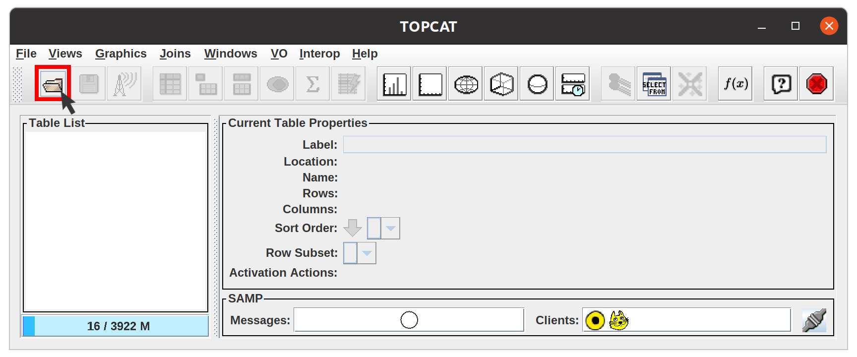
In TOPCAT, open a new table:
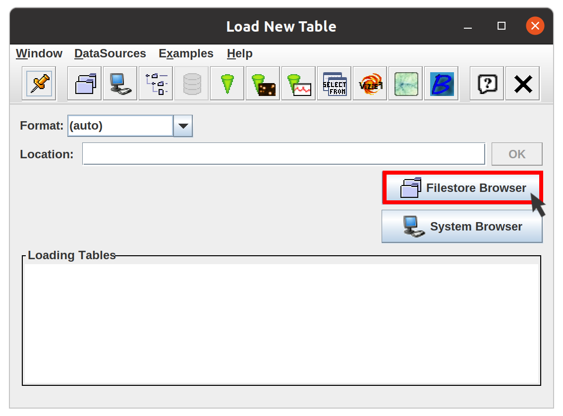
A new window will open. Click on Filestore Browser:
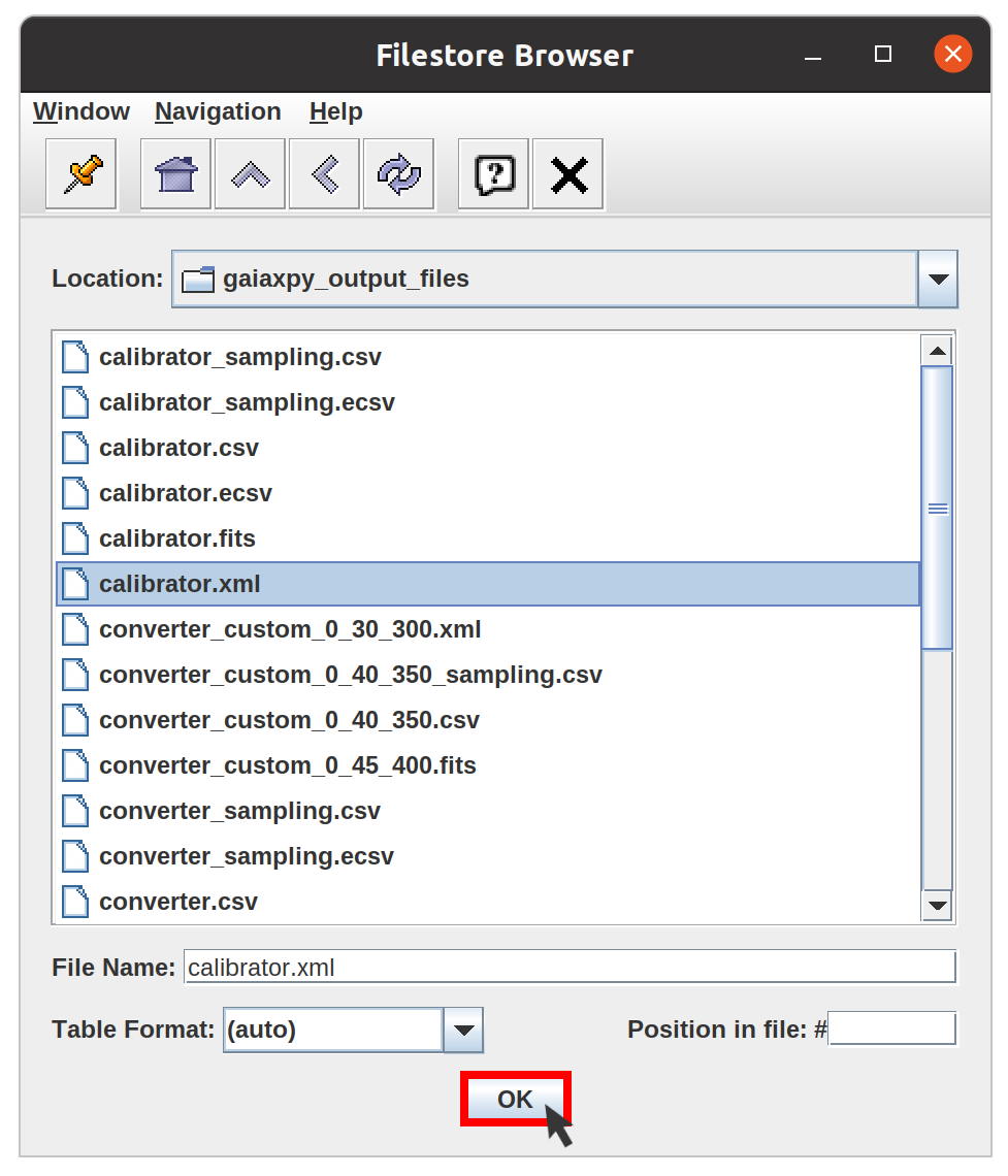
Navigate and select the file you want to open, then click OK:
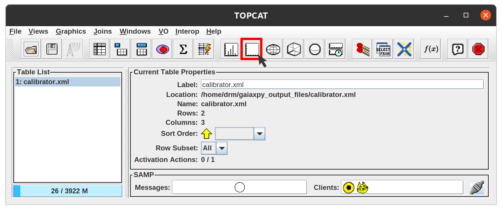
You should see you table in the Table list. Click on "Plane plotting window":
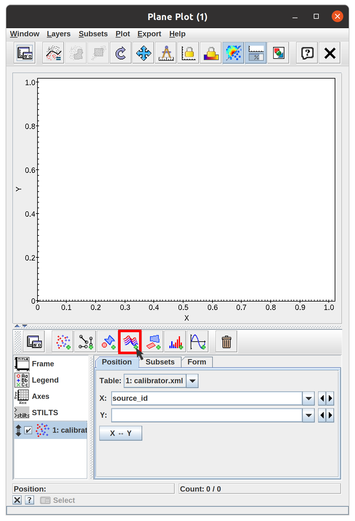
Click on "Add a new array pair plot control to the stack". Since only arrays and not points are being plotted, you should also uncheck the position layer control that it appears below.
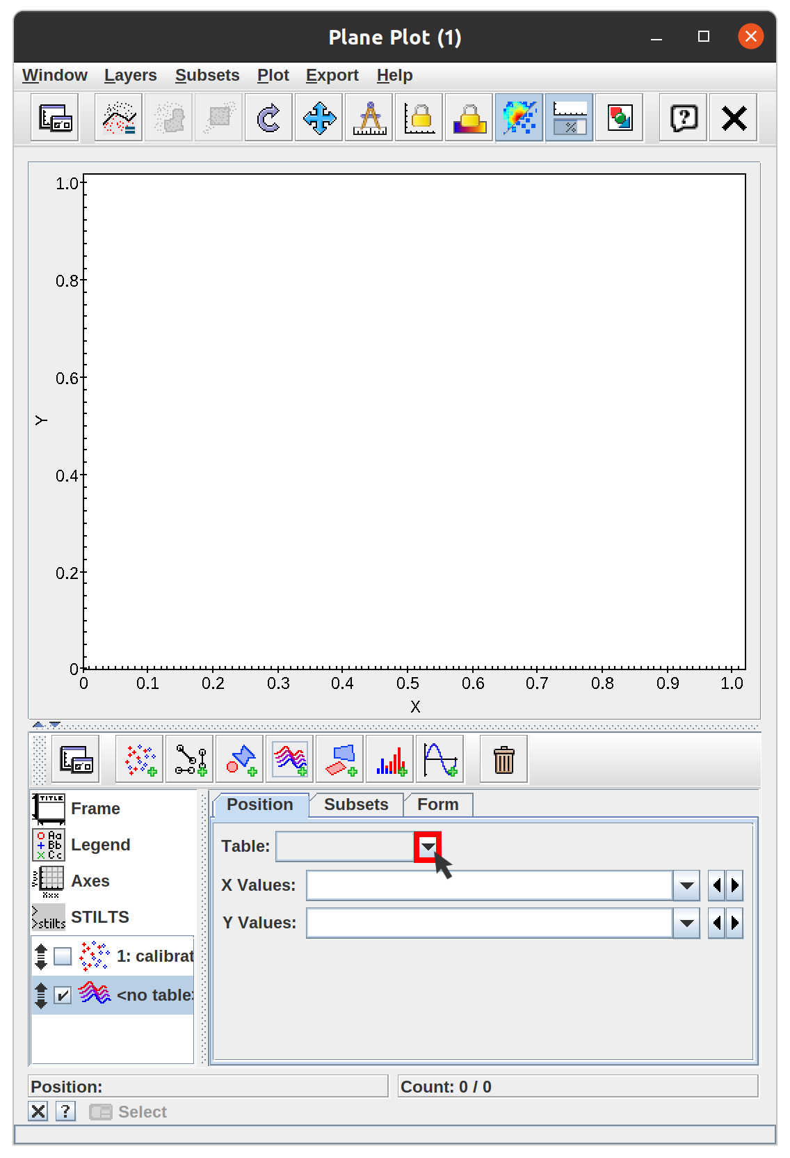
Select the table you want to plot:
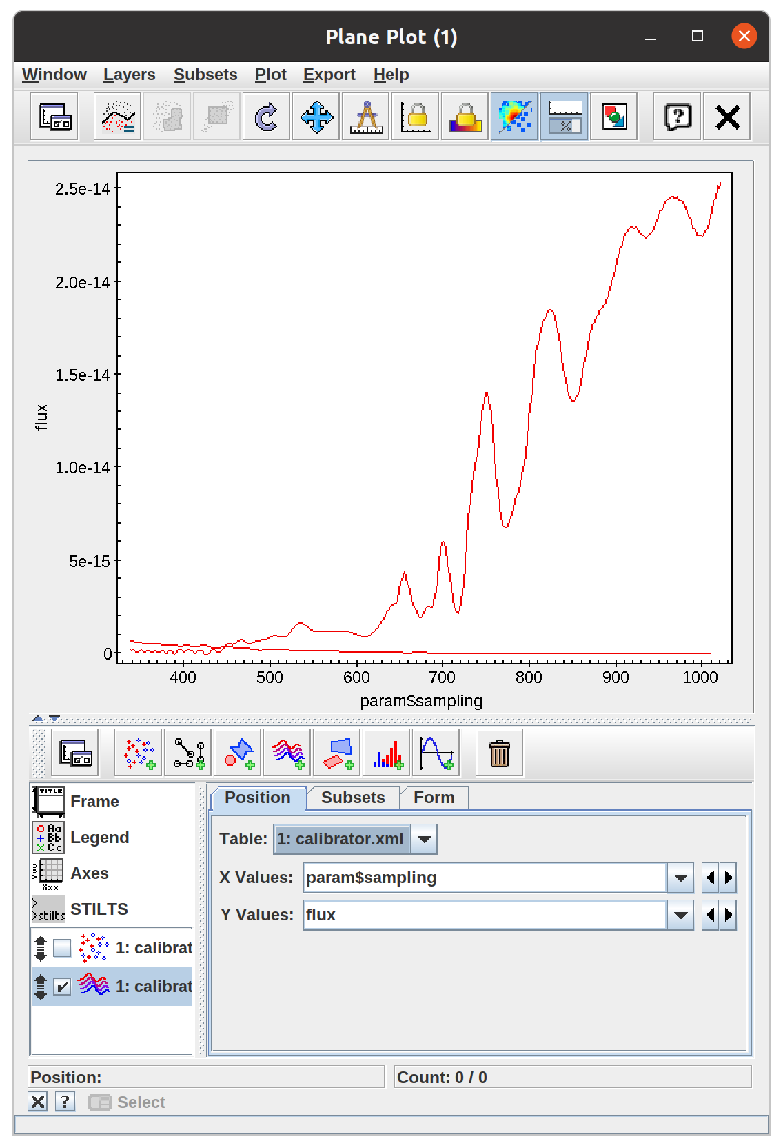
TOPCAT will automatically select the right parameters to create a spectra plot:
You can also generate plots from the command line using STILTS. A convenient way to do this is to set the plot up in TOPCAT and then use the STILTS control to display a command which you can use and adjust to taste. Some examples are below.
Plot flux spectra:
stilts plot2plane in=calibrator.fits xs='param$sampling' ys=flux layer1=lines
Plot spectra with errors:
           stilts plot2plane in=calibrator.fits xs='param$sampling' ys=flux
                  layer1=lines
                  layer2=yerrors yerrhis=flux_error
TOPCAT and STILTS include a powerful expression language that allow you to plot (and otherwise make use of) values obtained from columns in the table, as well as the column values themselves. For working with spectral data, a number of functions are provided to operate on arrays; documentation can be found in the Arrays class section of the manual or browsed under "Arrays" in TOPCAT's Available Functions Window. Some examples of expressions involving GaiaXPy-type arrays are:
multiply(param$sampling, 10.0)
multiply(reciprocal(param$sampling), C_KMS*1e12)
add(flux, flux_error)
multiply(flux, 1./mean(flux))
arrayFunc("log10(x)", flux)Expressions like these can be typed directly into the plotting window coordinate fields or used to create new columns. More examples can be found in the documentation, as above.